Statistics is a critical component of data science and machine learning algorithms. Almost all the machine learning algorithms use mathematics in the backend, which is linear algebra and statistics. Learning and understanding the core intuition and the working mechanisms of any machine learning algorithm requires a core knowledge of statistics.

In this article, we will discuss the famous statistic topic of measures of dispersion, which is being used to get an idea about the variance or spread of the data. Here we will discuss the range, inter-quartile range, variance, and standard deviation. Knowing about these key concepts in statistics will help one understand the machine learning algorithms better and answer the questions related to them with the logical backing of the statistics.

Let us start the discussion by answering the basic and common question, “What are measures?”

Table of Content

Measures of Central Tendency
Mean
Median
Mode
Measures of Dispersion
Range
InterQuartile Range
Variance
Standard Deviation
5 Key Points to Remember
Conclusion

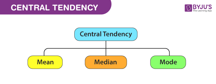
Measures of Central Tendency

Measures of tendency are the measures where a single value represents the whole dataset. The mean and median are used as the measures of central tendency. 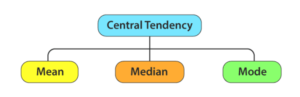Image Source

To calculate the “mean” of the data:

The mean is calculated by dividing the total observations by the sum of all the observation values.

Code:

mean = df['ColumnName'].mean()

To calculate the median:

List down all integers in ascending or descending order.
If the observations are odd, then the middle observations are treated as the median of the data.
If the observations are even, then the mean of the middle two observation values will be treated as the median of the data.

Code:

median = df['ColumnName'].median()

It is the most frequent category occurring in the dataset. It is used in categorical datasets. For example, if a column has 70 observations of yes and 30 observations of no, then the mode would be yes.

Note: In the case of the outlier, the mean is the most affected measure among all, as the outlier is going to have very high or low values, which will make the mean biased to one side. So in such cases, the median is preferred over the mean.

Measures of Dispersion in Statistics

Statisticians use dispersion measures to describe the spread or variance of a given dataset. These measures help statisticians understand the range of the data and the type of data present. Statisticians can get some insights from the data and can help them to know some common machine learning problems, such as the presence of outliers, by knowing the spread of the data.

Some measures used in statistics are:

Range
Interquartile Range
Variance
Standard Deviation

1. Range

The range is the difference between the smallest and largest value present in the dataset. This parameter helps one understand the normal range of the data and gives a basic overview of the type of data present.

Largest Value- Smallest Value = Range

Examples:

Data: 1, 2, 3, 4, 5

Range = 5 - 1 = 4

Data: 1, 4, 9, 2, 5

Range = 9 - 1 = 8

Data: 8, 7, 9

Range = 9 - 7 = 2

Code:

df.describe()

2. Inter Quartile Range (IQR)

The interquartile range represents the variability of a dataset based on its quartile division.

Before understanding the interquartile range, we need to understand the percentile. The percentile is a value below which a certain percentage of observations lie. For example, the 99 percentile means 99 percent of the observation values lie before this current value. If a student gets a 99 percentile in exams, it means that 99 percent of students have fewer marks than this student.

Image Source

The formula for the percentile is:

Percentile = number of values less than the given number divided by the total number of values

Now let’s try to understand the quartile.

The quartile divides the rank-ordered data into four equal sets of data. The subset of the data is now called the first, second, and third quartiles. They are denoted by Q1, Q2, and Q3, respectively.

Where,

Q1 = 25th Percentile

Q2 = 50% of the population = Median

Q3 = 75th Percentile

The interquartile range would be the value we get by subtracting the 25th percentile from the 75th percentile.

Inter Quartile Range = Q3 - Q1

Code:

Q3 = np.quantile(df[col], 0.75)
Q1 = np.quantile(df[col], 0.25)
IQR = Q3 - Q1

Now to remove the Outliers using IQR, use the code below:

# Removing the outliers
def removeOutliers(df, col):
    Q3 = np.quantile(df[col], 0.75)
    Q1 = np.quantile(df[col], 0.25)
    IQR = Q3 - Q1
    print("IQR value for column %s is: %s" % (col, IQR))
    global outlier_free_list
    global filtered_data
    lower_range = Q1 - 1.5 * IQR
    upper_range = Q3 + 1.5 * IQR
    outlier_free_list = [x for x in df[col] if (
        (x > lower_range) & (x < upper_range))]
    filtered_data = df.loc[df[col].isin(outlier_free_list)]

for i in df.columns:
    if i == df.columns[0]:
    removeOutliers(df, i)
else:
    removeOutliers(filtered_data, i)

df = filtered_data
print("Shape of data after outlier removal is: ", df.shape)

3. Variance

The variance is the spread of the dataset given. It is not much of a difference between the variant and the deviation. The squared values of deviations are known as the variance of the data. 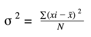Image Source

Where,

Sigma denotes the standard deviation.

Xi = the data’s ith element

Xbar = Observational Mean

N is the number of observations.

To get the variance of the column in the data frame, use the code below:

print(df.var()['Column'])

To plot a graph, use the code below:

import matplotlib.pyplot as plt
% matplotlin inline
plt.plot(df['Column'].var())

4. Standard Deviations

Standard deviations are the square root of the variance and can be computed by simply calculating the square root of the variance of the data. Image Source

The formula for standard deviations would be:

Image Source

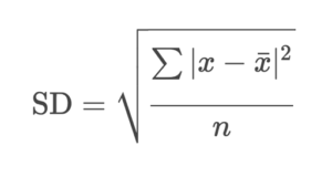
Code:

import pandas as pd
import numpy as np
import matplotlib.pyplot as plt
%matplotlib inline
print(df['column'].std())
plt.plot(df['column'].std())

Key Points to Remember (To deal with Outliers)Key Points to Remember (To deal with Outliers)

1. First Quartile (Q1)

The first quartile is the 25th percentile of the dataset and is denoted by Q1.

2. Second Quartile (Q2)

The second quartile is denoted as Q2, which is the 50th percentile of the values of the data.

3. Third Quartile (Q3)

The third quartile is the 75th percentile of the dataset and is denoted by Q3.

4. Lower Limit (LL)

The lower limit is the smaller integer present in the dataset.

Observations having values less than the lower limits are treated as outliers.

Lower Bound = Q1-1.5 IQR

5. Upper Limit (UL)

The upper limit is the largest integer present in the dataset.

Observations having values Outliers are those who exceed the upper limits.

Upper Limit = Q3 + 1.5 IQR

Conclusion

In this article, the measures of the dataset in statistics are discussed with their core intuitions, working mechanisms, and mathematical formulations. Knowing these core concepts will help one better understand and deal with machine learning algorithms. The five key points at the end of the article will also help one better understand the presence of outliers and how to treat them using these statistical measures.

Some Key Takeaways from this article are:

The mean and median are a measure of tendency, while the range, variance, IQR, and standard deviations are measures of dispersion.
The interquartile range is the difference between the 75th and 25th percentiles of the data, which divides the dataset into four equal subsets.
Variance describes the spread of the dataset, whereas the standard deviation is the square value equal to the amount of variance.
Values above the upper limit and below the lower limit are treated as outliers. They are either dropped or imputed using different techniques.